Every year, the NBA draft acts as the major pipeline for college players to turn professional by entering the NBA. A total of 60 players are selected; 30 being drafted during the first and second round respectively with their player rights being given to the team that made the selection. However, with there being several hundred players entering their name into the NBA draft, there still remains a massive pool of undrafted players available for any team to sign as a rookie free agent. In the past, NBA teams would be satisfied with just their draft picks because a team had a limited number of roster spots available. They also had a limited amount of scouting resources which ultimately were used on the top prospects. Lastly would not be able to find enough playing time to develop draft picks and rookie signings.
The hypothesis is that there exists more than 60 players every year that can potentially provide above replacement1 value for an NBA team. Using a statistical model using real-world player data, we propose a model that can be created to help identify these players of value.
The recent affiliation of the G-League (the official NBA development league) with the NBA gives us the opportunity to test this hypothesis. The G-League acts as a minor league for NBA teams with each major nba team having a development team. For example, the Toronto Raptors (NBA team) corresponding G-League development team is the Raptors 905. Essentially, an NBA teams corresponding G-League team doubles the available roster spots an NBA team has. Teams now have the ability to stash prospects in their development system (G-League team) and give these players time to develop. The NBA draft provides an average of two prospects to each team which is not enough to satisfy the new demand since teams can take on more prospects now. It is in a team’s best interest to sign as many low end prospects as possible because the cost versus potential upside favors teams in addition to failed players being easily cut from the team.
Currently, teams fill out their G-League roster spots by holding tryouts where unsigned players are tested and if they perform well enough, can make the G-League team. This method of finding players does not maximize the value of these draft spots because teams using their limited scouting resources are inviting certain players to show up at tryouts, when in reality there could be several dozen players that would be worth an evaluation.
A model was created to provide data on which players can provide value above replacement level from which teams can then specifically target if they are still available after the draft to see if it is worthwhile to introduce said players into their system.
To be clear, the model does not provide projections on players so it should not be used as a tool to decide who to draft. Draft picks are extremely valuable and scouts should be tasked on making such large decisions. Human evaluation of talent by scouts will always be better than a statistical model at projecting players and every player that may be drafted has been so heavily scouted that a statistical model cannot provide further insight.
However, the model will look at the lower end players who are not scouted and act as a supplementary tool used to bring attention to worthwhile players. The beauty of the model and machine learning algorithms in general is the massive amounts of data it can quickly analyze and make predictions on. Teams do not have the resources to scout every college player in detail so this model will act as a tool to help scouts identify which players outside of the top 60 projected draftees are worth taking a look.
There are much fewer centers than other positions because teams typically have one center, two guards and two forwards on the court. In addition, there are very few humans in the world tall enough to play the center position for this reason there is usually lower turnover for the position.
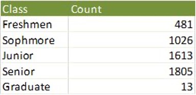
The number of players increases as the class increases because older players tend to be better and therefore get more playing time and more chances to make a team.
Figure 2: Distribution of players by Class
In the data 3.6% of all players end up being drafted to an NBA team. The average strength of schedule of the players included in the data is 0.358, showing that the data set is slightly skewed towards players in higher end conferences. Players from these conferences are more likely to be drafted anyways so it makes sense to skew the data is this direction.
There have been 4,952,315 minutes played overall across all players in the data. This puts into perspective the sheer magnitude of the data analyzed by the model and how it would be impossible for a team to get scouts to do the analysis by purely watching games.
Results
The purpose of this project was to predict whether or not a player in the NCAA had the abilities and necessary skills to provide value in the NBA. As such, the class variable was whether or not the NCAA player was drafted or not. The binary class variable, Drafted, was used to determine this classification.
Supervised Learning
The supervised learning portion of the project required the usage of classification machine learning algorithms such as: KNN, Logistic Regression, Decision Trees, and Naive Bayes. Through running the data through these algorithms a dashboard of statistics were determined, these statistics were then compared to find the ideal algorithm which produced the most accurate results.
False Positive vs. False Negative
All models are inherently incorrect; through this understanding, the model must be evaluated even when it produces false positive and negative results. When the algorithm provides a false positive result it is essentially finding athletes who the algorithm classifies as being drafted even though they were not. False negative represents the athletes which the algorithm classified as not making the draft, even though they were drafted. As this tool is one which is meant to help scouts in their job to find potential candidates to draft, having a higher false positive rate is more beneficial and less costly than a higher false negative. This is due to the fact that when provided athletes who would not be drafted a scout can easily discern this and discount the athlete.
However, is a possible candidate is not identified, it may result in loss of profits for the NBA and loss of commission to the scout. Therefore to reduce cost algorithms with higher false positive results are more economical than algorithms with higher false negative results.
K-Folds Validation
K-Folds validation was done on each supervised learning method with the k value set to 10. Due to the nature of the class variable, k-folds validation yielded a high accuracy for every one of the methods. The reason for this is because the class variable is overwhelming skewed towards one value and any model will classify the large majority of players to be undrafted leading to a high accuracy. Accuracy is not a good statistic to use to judge the goodness of each model making K- Folds validation not a good way to evaluate the model. An accuracy of 100% will actually not be ideal because that will not provide insight to scouts on who to target after the draft is over.
KNN
K-Nearest Neighbour is a non-parametric means of classifying data which uses distance to determine the value of the output. KNN is one of the most simple algorithms which can be used for classification. The dataset was passed through a KNN algorithm and the following dashboard and confusion matrix was discovered.
Figure 3: Confusion matrix and Dashboard for KNN
Solely observing the accuracy of the KNN algorithm provides a very misleading representation of the real accuracy of the classifier. Due to the fact that there are many more “NO” classifications than the “YES” classification the accuracy is skewed. However, looking at the true positive rates, false positive rates, and misclassification rate give a more well rounded and accurate representation of the model. Comparing all the values, KNN is very clearly seen to be a less than desirable model as it has a low true positive rate and a low false positive rate with a very high false negative rate.
It only predicts a total of 64 drafted players over the five year period when in reality 180 were drafted. This means that the model only selected the top end players to be drafted and scouts already know who the best players are without the help with a model. Such a low pYES number is unlikely to be able to provide any insight to scouts on who to sign after the draft which is the purpose of the model.
Decision Trees
Decision trees build classification models which uses a tree-like graph. At the nodes of the tree it maps decisions while giving it’s possible consequences. The objective of a decision tree is to develop rules and decisions which take data and parse it to determine a classification. The dataset of NCAA players were passed through a decision tree model and the following dashboard and confusion matrix was determined:
Figure 4: Confusion matrix and Dashboard for Decision Trees
At first glance the decision tree model is almost entirely accurate. However, through further inspection is was clear that the decision tree was severely overfitting the model to the data. In fact, the extent of the overfitting was so severe that the decision tree created contained specific rules for every single instance of the positive instance in the binary class variable (See Appendix A for the decision tree visualization). Although pruning and other methods exist to reduce overfitting it was found through iterations of testing that the level of overfitting in decision trees were too high to be useful in providing useful conclusions. As such the decision tree model was disregarded as a means to classify NCAA players accurately.
Logistic Regression
Logistic regression is a categorical regression model; it is a means of defining the likelihood that a the class variable will be either a one or zero. Using a logit function the logistic regression model issues weights to explanatory variables and maps this to the logit function. Using a linear discriminator the logistic regression model classifies an input as either a one or a zero. Passing the NCAA data through the logistic regression model the following dashboard, and confusion matrix was determined:
Figure 5: Confusion matrix and Dashboard for Logistic Regression
Although better than the previous two models the logistic regression model has a very high false negative rate. This means that players who were drafted would not have been predicted to be drafted. This oversight of the model does not provide insight to scouts. As mentioned previously a successful model is one which somewhat accurately predicts the athletes who will get drafted and also more who should’ve been drafted. The model should have more false positives than negatives if the case arises to reduce the possibility of overlooking potential NBA talent . As this model does not minimize false negatives, it is not fit to be used as the model of choice to determine future NBA draft picks.
Naive Bayes
The naive bayes model is a classification model which uses likelihood estimates of the dataset to determine the classification of an input. As the data provided in the dataset is primarily numeric, and continuous data points the naive bayes algorithm creates normal distributions on each column when learning. Applying these distributions to the input, the algorithm determines how to classify the input. The NCAA dataset was passed through the naive bayes model and the following dashboard and confusion matrix was determined:
Figure 6: Confusion matrix and Dashboard for Naive Bayes
Barring the decision tree model the naive bayes model has the highest number of correctly predicted athletes who get drafted. The false positive value of the model is higher than the false
negative; this creates value in terms of accounting for value which would have been lost with a higher false negative rate. The high true positive rate also depicts the usefulness of this model compared to the previous three. Aggregating all the positives of this model, it can be determined that this model is one which most accurately and economically predicts the athletes who have the potential to get drafted for the NBA.
Naive bayes yields a larger “YES” value than the actual. This great because it is able to find useful NBA players outside of the draft. An analysis of the results of Naive bayes found that out of the 687 predicted yes values 41 were undrafted players who eventually made it to the NBA. Naive bayes was able to identify useful undrafted players such as Robert Covington, Tim Frazier, Matthew Dellavedova, and Kent Bazemore. This ability makes it a valuable tool. Robert Covington is projected to produce over 27 million dollars of value this year[2] yet will only be paid a bit more that 1.5 million [6]. The fact that the naive bayes model is able to find such a player makes it extremely valuable.
The reason naive bayes model produces so many more false positives than other models is because it utilizes the naive assumption that features in the model are normally distributed. However, at the highest competitive level of NCAA the differences between drafted players and good players are miniscule.. Consider the fact that the difference in FG% between a great and average player would be around 5%, the marginal difference between a good and great player is even smaller. Since the naive bayes model is unable to make such small distinctions it ends up making predictions liberally.
Compare and Contrast
As stated previously a higher number of false positives is desirable as it is the data that will result in finding useful undrafted players from the NCAA. Looking at the four models detailed above it is clear the only one with a desirable number of false positives is the naive bayes model. The other models are essentially useless because it cannot provide that same insight. The decision tree model overfit the data to a level where it was not translatable to other models.
To further understand the effect of the models on data it has not seen, testing was done on a set of test data the models had never seen (see Appendix D). From this test it is clear that the naive bayes is superior other models created. It predicts the highest number correctly, while providing a higher false positive through which the scouts can comb through and find draftable players.
Clustering
Clustering was done on the entirety of the dataset with FG, TRB% and AST% on the axises. These three data items were chosen because scoring, rebounds and assists are the three most looks at statistics in the NBA and in college basketball. It is evident by the popularity of the triple
double3 as a talking point in the media. Clustering resulted in 3 clusters with different skillsets (Refer to Appendix B).
Looking at the clusters in Appendix B; the teal cluster represents players who score a high number of field goals but do not contribute heavily in terms of rebounds and assists. The purple cluster contains specialists who do not score much but contribute by having a high number of rebounds and/ or assists. Finally there is a yellow cluster which consists of unskilled players who do not contribute much in any aspect. In the NBA nearly every player is able to contribute in some way but in college there is a much more diluted talent pool and there will be a large number of players who are not skilled enough to contribute.
Clustering was also done with the same axises on only the drafted players and it provided an interesting insight. There ended up being three clusters with distinctly different skillsets. The teal cluster contained high scoring players with high rebound rates. These are likely very tall centres or power forwards who at the college level could score with ease. The variance of height is much higher in college basketball and large players have much more of an advantage than they do in the NBA. Due to their physical gifts, they are very strong at scoring and rebounding. The next cluster is the purple cluster which contains low scoring players with high rebound rates or high assist rates but not both. These players are specialists who are either great at rebounding or playmaking and they are drafted by nba teams who have a need for that one skillset. Lastly the yellow cluster consists of pure scorers. These players make a lot of field goals but do not rebound or assist much. Scoring is inherently valuable in basketball and teams will always value scoring. These are also likely to be average or shorter players evident by the low rebound rates. They rely more heavily on skill to score unlike their teal cluster counterparts who rely more on their physical stature to score.
Conclusions
Through comparing and contrasting different methods of classification through supervised learning, it is abundantly clear that naive bayes provides the best results for this instance of analysis. By introducing NCAA data to the model, it has successfully determined players who were drafted as well as identified players who were not drafted but eventually got into the NBA and had successful. The model was designed to help NBA scouts and NBA teams identify lower end player available after the draft to look into and its ability to identify cheap talent will help NBA teams greatly.